DCF: An Efficient and Robust Density-Based Clustering Method

Mimi Zhang [ https://orcid.org/0000-0002-3807-297X ]

This notebook introduces the DCF algorithm for cluster analysis.

Introduction

DCF is the acronym for density-core finding, an improvement on the popular density-peak clustering (DPC) method. The DPC method detects modes as points with (1) high density and (2) large distance to points of higher density. Hence, it often fails to adequately represent clusters with areas of relatively uniform density.

DCF is both efficient and robust, gracefully scaling to big datasets. The improvements offered by DCF are twofold:

• the algorithm is robust to noise in the density estimate and thus detects clusters at varying densities;
• the algorithm is competent at deciding the correct number of clusters, even when the number of clusters is very high.

The improvements are the result of directing the peak-finding technique to discover modal sets, rather than point modes.

The Algorithm

The DCF algorithm consists of the following main steps:

(1) Compute the peak-finding criterion for each data point and select the instance $\mathbf{x}$ with maximal value.

(2) The component set $\mathbf{S}_{\beta}(\mathbf{x})$ containing $\mathbf{x}$ is the first cluster core. All points in $\mathbf{S}_{\beta}(\mathbf{x})$ are labelled with $Assessed$ and excluded from further consideration.

(3) The instance $\mathbf{x}$ with maximal value of the peak-finding criterion, yet to be assessed, is selected.

(4) The component set $\mathbf{S}_{\beta}(\mathbf{x})$ containing $\mathbf{x}$ is found.

• All points in $\mathbf{S}_{\beta}(\mathbf{x})$ are labelled with $Assessed$ and excluded from further consideration.
• $\mathbf{S}_{\beta}(\mathbf{x})$ is another cluster core only if it is disjoint from all previously detected cluster cores.

(5) Repeat Steps 3 and 4 until all points have been labelled with $Assessed$.

Each cluster core represents a different cluster, and the number of detected cluster cores is the number of clusters in the data. After Step 5, there will be many data points that are labelled with $Assessed$ but do not belong to any cluster core set. These non-core points are from the component sets $\mathbf{S}_{\beta}(\mathbf{x})$ in Step 4 that overlap with previously detected cluster cores.

(6) Each non-core point is assigned to the same cluster as its nearest neighbor of higher density.

DCF uses the peak-finding criterion of DPC to detect cluster cores. The peak-finding criterion is computed for each data point, and the instance with maximum value is selected as a center (Step 1). The cluster core containing this center is then found, and all instances belonging to it are removed from consideration as potential centers (Step 2). The algorithm continues detecting cluster cores until no more remain in the data (Steps 3-5). The allocation procedure is unchanged from the DPC method: each non-center point is allocated to the same cluster as its nearest neighbor of higher estimated density (Step 6).

The Two Inputs

The algorithm requires two user inputs: the neighborhood parameter $k$ (for density estimation) and the fluctuation parameter $\beta$ (for determining how much the density estimates can vary within a cluster core). In particular, the algorithm adopts a non-parametric density estimator: for any data point $\mathbf{x}\in\mathrm{R}^d$, its density estimate is \begin{equation*} \hat{f}(\mathbf{x})=\frac{k}{\mbox{sample size}\times \mbox{volume of the unit sphere in } \mathrm{R}^d \times r_k(\mathbf{x})^d}, \end{equation*} where $r_k(\mathbf{x})$ is the distance between $\mathbf{x}$ and its $k$th nearest neighbor in $\mathcal{X}$. For a user, specifying the value $k$ is much easier than specifying the cutting-off distance value in the DPC algorithm.

The definition of cluster core depends on the notion of mutual $k$-NN graph. Let $G$ denote the undirected mutual $k$-NN graph constructed from the whole dataset $\mathcal{X}$. (There is an edge between two vertices in $G$, if and only if they are one (out of $k$) nearest neighbor of each other.) We here explain how the first cluster core in Step 2 is determined. Let $\mathbf{x}^*$ be the point with the maximal value of the peak-finding criterion. Then the subset $S=\{\mathbf{x}\in\mathcal{X}: \hat{f}(\mathbf{x})\geq (1-\beta)\hat{f}(\mathbf{x}^*)\}$ contains all the data points with their density estimate ranging in the interval $[(1-\beta)\hat{f}(\mathbf{x}^*), \hat{f}(\mathbf{x}^*)]$. The subset $S$ determines a sub-graph of $G$:

• The vertices of the sub-graph are the data points in $S$.
• There is an edge between two vertices in the sub-graph, only if there is an edge between them in the original graph $G$.

Then the cluster core $\mathbf{S}_{\beta}(\mathbf{x}^*)$ is simply the connected component of the sub-graph that contains the point/vertex $\mathbf{x}^*$.

Point Modes vs Cluster Cores

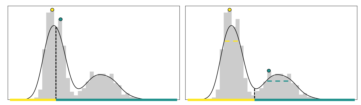
An illustrative example demonstrating the benefits of seeking cluster cores of the density. The black curve represents the underlying density and the grey histogram represents a sample from the density. Left: DPC incorrectly selects both centers from the first cluster, as the noise in the density estimate causes the peak-finding method to favor the high-density cluster. Right: Cluster cores, represented by dashed lines, better represent the cluster centers.

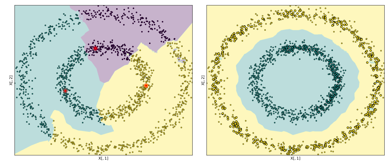
Comparison of the DPC and DCF methods when applied to the Noisy Circles dataset. The Noisy Circles dataset contains two clusters, a high-density cluster (inner circle) and a low-density cluster (outer circle). The DPC method, as seen on the left of the figure, proceeds by searching for the points with maximal values of the peak-finding criterion. This method erroneously selects the multiple centers from the inner cluster. The allocation mechanism incorrectly assigns all points in the outer cluster. For this example, seven points in the inner cluster have larger value of the peak-finding criterion than the maximum value in the outer cluster.

The DCF procedure can be seen on the right of the figure. We first select the instance of maximum density as the first peak. However, DCF proceeds to compute the cluster core associated with this point, the highlighted larger green points, and remove all elements of the core from consideration as centers. Of those remaining, the point with maximal value of the peak-finding criterion is in the outer cluster. The associated cluster core is visible in yellow. As no edge in the $k$-NN graph exists between this cluster core and the first cluster core, it is accepted as a valid cluster core. The algorithm's termination procedure is invoked when assessing a third center. The third center is selected as before; however, as the cluster core associated with this point contains all of the instances in the dataset, the algorithm terminates.

Code Examples

The code examples below were mainly contributed by Sachit Bhardwaj.

# Import libraries.

import sys
sys.path.insert(1, './src')
import numpy as np
import pandas as pd
from DCFcluster import DCFcluster
from itertools import cycle, islice
import matplotlib.pyplot as plt
from matplotlib.collections import LineCollection
import warnings
from sklearn import cluster, datasets, metrics

# Simulate synthetic datasets.

np.random.seed(0)
n_samples = 1500

noisy_circles = datasets.make_circles(n_samples=n_samples, factor=.5, noise=.05)

half_moons = datasets.make_moons(n_samples=n_samples, noise=.05)

blobs = datasets.make_blobs(n_samples=n_samples, random_state=8)
X, y = datasets.make_blobs(n_samples=n_samples, random_state=170)
transformation = [[0.6, -0.6], [-0.4, 0.8]]
X_aniso = np.dot(X, transformation)
aniso = (X_aniso, y)

varied = datasets.make_blobs(n_samples=n_samples, cluster_std=[1.0, 2.5, 0.5], random_state=170)

Example 1

# Plot the noisy_circles dataset.

Data = noisy_circles
X = Data[0]
y = Data[1]
plt.xlim(X[:,0].min(), X[:,0].max())
plt.ylim(X[:,1].min(), X[:,1].max())
plt.scatter(X[:, 0], X[:, 1], s = 1,marker = "o")
plt.xticks(())
plt.yticks(())

([], [])

# Apply the DCF algorithm on the dataset and visualize the clustering results.

result = DCFcluster.train(X, k = 40, beta = 0.4)

colors = np.array(list(islice(cycle(['#377eb8', '#ff7f00', '#4daf4a','#f781bf', '#a65628', '#984ea3',
                                    '#999999', '#e41a1c', '#dede00']), int(max(result.labels) + 1))))
plt.xlim(X[:,0].min(), X[:,0].max())
plt.ylim(X[:,1].min(), X[:,1].max())
plt.scatter(X[:, 0], X[:, 1], s = 1,color = colors[result.labels],marker = "o")
plt.text(.99, .01, ('k= {0} beta= {1}'.format(str(40), str(0.4))).lstrip('0'),
                 transform=plt.gca().transAxes, size=15,
                 horizontalalignment='right')
plt.xticks(())
plt.yticks(())

([], [])

Example 2

# Plot the varied dataset.

Data = varied
X = Data[0]
y = Data[1]
plt.xlim(X[:,0].min(), X[:,0].max())
plt.ylim(X[:,1].min(), X[:,1].max())
plt.scatter(X[:, 0], X[:, 1], s = 1,marker = "o")
plt.xticks(())
plt.yticks(())

([], [])

# Apply the DCF algorithm on the dataset and visualize the clustering results.

result = DCFcluster.train(X, k = 40, beta = 0.4)

colors = np.array(list(islice(cycle(['#377eb8', '#ff7f00', '#4daf4a','#f781bf', '#a65628', '#984ea3',
                                    '#999999', '#e41a1c', '#dede00']), int(max(result.labels) + 1))))
plt.xlim(X[:,0].min(), X[:,0].max())
plt.ylim(X[:,1].min(), X[:,1].max())
plt.scatter(X[:, 0], X[:, 1], s = 1,color = colors[result.labels],marker = "o")
plt.text(.99, .01, ('k= {0} beta= {1}'.format(str(40), str(0.4))).lstrip('0'),
                 transform=plt.gca().transAxes, size=15,
                 horizontalalignment='right')
plt.xticks(())
plt.yticks(())

([], [])

Example 3

# Plot the aniso dataset.

Data = aniso
X = Data[0]
y = Data[1]
plt.xlim(X[:,0].min(), X[:,0].max())
plt.ylim(X[:,1].min(), X[:,1].max())
plt.scatter(X[:, 0], X[:, 1], s = 1,marker = "o")
plt.xticks(())
plt.yticks(())

([], [])

# Apply the DCF algorithm on the dataset and visualize the clustering results.

result = DCFcluster.train(X, k = 40, beta = 0.4)

colors = np.array(list(islice(cycle(['#377eb8', '#ff7f00', '#4daf4a','#f781bf', '#a65628', '#984ea3',
                                    '#999999', '#e41a1c', '#dede00']), int(max(result.labels) + 1))))
plt.xlim(X[:,0].min(), X[:,0].max())
plt.ylim(X[:,1].min(), X[:,1].max())
plt.scatter(X[:, 0], X[:, 1], s = 1,color = colors[result.labels],marker = "o")
plt.text(.99, .01, ('k= {0} beta= {1}'.format(str(40), str(0.4))).lstrip('0'),
                 transform=plt.gca().transAxes, size=15,
                 horizontalalignment='right')
plt.xticks(())
plt.yticks(())

([], [])

Example 4

# Plot the half_moons dataset.

Data = half_moons
X = Data[0]
y = Data[1]
plt.xlim(X[:,0].min(), X[:,0].max())
plt.ylim(X[:,1].min(), X[:,1].max())
plt.scatter(X[:, 0], X[:, 1], s = 1,marker = "o")
plt.xticks(())
plt.yticks(())

([], [])

# Apply the DCF algorithm on the dataset and visualize the clustering results.

result = DCFcluster.train(X, k = 40, beta = 0.4)

colors = np.array(list(islice(cycle(['#377eb8', '#ff7f00', '#4daf4a','#f781bf', '#a65628', '#984ea3',
                                    '#999999', '#e41a1c', '#dede00']), int(max(result.labels) + 1))))
plt.xlim(X[:,0].min(), X[:,0].max())
plt.ylim(X[:,1].min(), X[:,1].max())
plt.scatter(X[:, 0], X[:, 1], s = 1,color = colors[result.labels],marker = "o")
plt.text(.99, .01, ('k= {0} beta= {1}'.format(str(40), str(0.4))).lstrip('0'),
                 transform=plt.gca().transAxes, size=15,
                 horizontalalignment='right')
plt.xticks(())
plt.yticks(())

([], [])

Example 5

Seed variety dataset consists of measurements of geometrical properties of kernels belonging to three different varieties of wheat. A soft X-ray technique and GRAINS package were used to construct all seven, real-valued attributes. The target class is dropped for the demonstration of the DCF algorithm. This dataset is widely available and downloaded from Kaggle

# Load dataset.

df = pd.read_csv('Seed_Data.csv')
df.head()

	A	P	C	LK	WK	A_Coef	LKG	target
0	15.26	14.84	0.8710	5.763	3.312	2.221	5.220	0
1	14.88	14.57	0.8811	5.554	3.333	1.018	4.956	0
2	14.29	14.09	0.9050	5.291	3.337	2.699	4.825	0
3	13.84	13.94	0.8955	5.324	3.379	2.259	4.805	0
4	16.14	14.99	0.9034	5.658	3.562	1.355	5.175	0

# Plot all the features.

import seaborn as sns
sns.lineplot(data=df.drop(['target'], axis=1))
plt.show()

df.columns

Index(['A', 'P', 'C', 'LK', 'WK', 'A_Coef', 'LKG', 'target'], dtype='object')

X = df[['A', 'P', 'C', 'LK', 'WK', 'A_Coef', 'LKG']]     

# Standardize the features by subtracting the mean and then scaling to unit variance.

from sklearn.preprocessing import StandardScaler
scale = StandardScaler()
scale.fit(X)
X_scaled = scale.transform(X)

# Apply the DCF algorithm on the dataset and visualize the clustering results.

result = DCFcluster.train(X_scaled, k = 14, beta = 0.7)

# Visualize through columns 1 and 2.

colors = np.array(list(islice(cycle(['#377eb8', '#ff7f00', '#4daf4a','#f781bf', '#a65628', '#984ea3',
                                    '#999999', '#e41a1c', '#dede00']), int(max(result.labels) + 1))))
plt.xlim(X_scaled[:,0].min(), X_scaled[:,0].max())
plt.ylim(X_scaled[:,1].min(), X_scaled[:,1].max())
plt.scatter(X_scaled[:, 0], X_scaled[:, 1], s = 1,color = colors[result.labels],marker = "o")
plt.text(.99, .01, ('k= {0} beta= {1}'.format(str(14), str(0.7))).lstrip('0'),
                 transform=plt.gca().transAxes, size=15,
                 horizontalalignment='right')
plt.xticks(())
plt.yticks(())

([], [])

Three clusters were detected.

# pairwise scatter plot

def matrix_plot(a,b,c):
    colors = np.array(list(islice(cycle(['#377eb8', '#ff7f00', '#4daf4a','#f781bf', '#a65628', '#984ea3',
                                    '#999999', '#e41a1c', '#dede00']), int(max(result.labels) + 1))))
    plt.xlim(X_scaled[:,a].min(), X_scaled[:,a].max())
    plt.ylim(X_scaled[:,b].min(), X_scaled[:,b].max())
    plt.subplot(2,2,c)
    plt.scatter(X_scaled[:, 0], X_scaled[:, 1], s = 1,color = colors[result.labels],marker = "o")
    plt.xticks(())
    plt.yticks(())

matrix_plot(1,2,1)
matrix_plot(2,3,2)
matrix_plot(3,4,3)
matrix_plot(4,5,4)
plt.show()

# AMI & ARI

ami = metrics.adjusted_mutual_info_score(df['target'].astype(int), result.labels.astype(int))
ari = metrics.adjusted_rand_score(df['target'].astype(int), result.labels.astype(int))
print("Adjusted Mutual Information Score -", ami)
print ("Adjusted Rand Score -", ari)

Adjusted Mutual Information Score - 0.7217366105244023
Adjusted Rand Score - 0.7847997819414604

# Sensitivity analysis w.r.t. k.

ari = np.zeros(5)
ami = np.zeros(5)

ari[0] = metrics.adjusted_rand_score(df['target'].astype(int), DCFcluster.train(X_scaled, k = 10, beta = 0.7).labels.astype(int))
ari[1] = metrics.adjusted_rand_score(df['target'].astype(int), DCFcluster.train(X_scaled, k = 11, beta = 0.7).labels.astype(int))
ari[2] = metrics.adjusted_rand_score(df['target'].astype(int), DCFcluster.train(X_scaled, k = 12, beta = 0.7).labels.astype(int))
ari[3] = metrics.adjusted_rand_score(df['target'].astype(int), DCFcluster.train(X_scaled, k = 13, beta = 0.7).labels.astype(int))
ari[4] = metrics.adjusted_rand_score(df['target'].astype(int), DCFcluster.train(X_scaled, k = 14, beta = 0.7).labels.astype(int))

ami[0] = metrics.adjusted_mutual_info_score(df['target'].astype(int), DCFcluster.train(X_scaled, k = 10, beta = 0.7).labels.astype(int))
ami[1] = metrics.adjusted_mutual_info_score(df['target'].astype(int), DCFcluster.train(X_scaled, k = 11, beta = 0.7).labels.astype(int))
ami[2] = metrics.adjusted_mutual_info_score(df['target'].astype(int), DCFcluster.train(X_scaled, k = 12, beta = 0.7).labels.astype(int))
ami[3] = metrics.adjusted_mutual_info_score(df['target'].astype(int), DCFcluster.train(X_scaled, k = 13, beta = 0.7).labels.astype(int))
ami[4] = metrics.adjusted_mutual_info_score(df['target'].astype(int), DCFcluster.train(X_scaled, k = 14, beta = 0.7).labels.astype(int))

x = [10,11,12,13,14]
default_x_ticks = range(len(x))
plt.plot(default_x_ticks, ami, color = "#9ecae1", marker = "o", label = "AMI")
plt.plot(default_x_ticks, ari,color = "#636363", marker = "o", label = "ARI")
plt.xticks(default_x_ticks, x)
plt.legend()
plt.ylabel("AMI/ARI")
plt.xlabel("neighborhood parameter k")
plt.show()

# Sensitivity analysis w.r.t. beta.

ari = np.zeros(5)
ami = np.zeros(5)

ari[0] = metrics.adjusted_rand_score(df['target'].astype(int), DCFcluster.train(X_scaled, k = 15, beta = 0.1).labels.astype(int))
ari[1] = metrics.adjusted_rand_score(df['target'].astype(int), DCFcluster.train(X_scaled, k = 15, beta = 0.3).labels.astype(int))
ari[2] = metrics.adjusted_rand_score(df['target'].astype(int), DCFcluster.train(X_scaled, k = 15, beta = 0.5).labels.astype(int))
ari[3] = metrics.adjusted_rand_score(df['target'].astype(int), DCFcluster.train(X_scaled, k = 15, beta = 0.7).labels.astype(int))
ari[4] = metrics.adjusted_rand_score(df['target'].astype(int), DCFcluster.train(X_scaled, k = 15, beta = 0.8).labels.astype(int))

ami[0] = metrics.adjusted_mutual_info_score(df['target'].astype(int), DCFcluster.train(X_scaled, k = 15, beta = 0.1).labels.astype(int))
ami[1] = metrics.adjusted_mutual_info_score(df['target'].astype(int), DCFcluster.train(X_scaled, k = 15, beta = 0.3).labels.astype(int))
ami[2] = metrics.adjusted_mutual_info_score(df['target'].astype(int), DCFcluster.train(X_scaled, k = 15, beta = 0.5).labels.astype(int))
ami[3] = metrics.adjusted_mutual_info_score(df['target'].astype(int), DCFcluster.train(X_scaled, k = 15, beta = 0.7).labels.astype(int))
ami[4] = metrics.adjusted_mutual_info_score(df['target'].astype(int), DCFcluster.train(X_scaled, k = 15, beta = 0.8).labels.astype(int))

x = [0.1,0.3, 0.5, 0.7, 0.8]
default_x_ticks = range(len(x))
plt.plot(default_x_ticks, ami, color = "#9ecae1", marker = "o", label = "AMI")
plt.plot(default_x_ticks, ari,color = "#636363", marker = "o", label = "ARI")
plt.xticks(default_x_ticks, x)
plt.legend()
plt.ylabel("AMI/ARI")
plt.xlabel("fluctuation parameter β")
plt.show()

Example 6

The wine quality dataset contains records related to red and white variants of the Portuguese Vinho Verde wine. It contains information from 1599 red wine samples and 4898 white wine samples. Input variables in the dataset consist of the type of wine (either red or white wine) and metrics from objective tests (acidity levels, PH values, ABV, etc.), while the target/output variable is a numerical score based on sensory data—median of at least 3 evaluations made by wine experts. Each expert graded the wine quality between 0 (very bad) and 10 (very excellent). This dataset is downloaded from UCI Machine Learning Repository

# Load dataset.

df = pd.read_csv('wine-quality-white-and-red.csv')
df.head()

	type	fixed acidity	volatile acidity	citric acid	residual sugar	chlorides	free sulfur dioxide	total sulfur dioxide	density	pH	sulphates	alcohol	quality
0	white	7.0	0.27	0.36	20.7	0.045	45.0	170.0	1.0010	3.00	0.45	8.8	6
1	white	6.3	0.30	0.34	1.6	0.049	14.0	132.0	0.9940	3.30	0.49	9.5	6
2	white	8.1	0.28	0.40	6.9	0.050	30.0	97.0	0.9951	3.26	0.44	10.1	6
3	white	7.2	0.23	0.32	8.5	0.058	47.0	186.0	0.9956	3.19	0.40	9.9	6
4	white	7.2	0.23	0.32	8.5	0.058	47.0	186.0	0.9956	3.19	0.40	9.9	6

# Plot the features.

import seaborn as sns
sns.lineplot(data=X)
plt.show()

We have to check for null values and replace them with zero.

df.isnull().sum()

type                    0
fixed acidity           0
volatile acidity        0
citric acid             0
residual sugar          0
chlorides               0
free sulfur dioxide     0
total sulfur dioxide    0
density                 0
pH                      0
sulphates               0
alcohol                 0
quality                 0
dtype: int64

df.columns

Index(['type', 'fixed acidity', 'volatile acidity', 'citric acid',
       'residual sugar', 'chlorides', 'free sulfur dioxide',
       'total sulfur dioxide', 'density', 'pH', 'sulphates', 'alcohol',
       'quality'],
      dtype='object')

X = df[['fixed acidity', 'volatile acidity', 'citric acid',
       'residual sugar', 'chlorides', 'free sulfur dioxide',
       'total sulfur dioxide', 'density', 'pH', 'sulphates', 'alcohol',
       'quality']] 

from sklearn import preprocessing
label_encoder = preprocessing.LabelEncoder()
df['type']= label_encoder.fit_transform(df['type'])

# Standardize the features by subtracting the mean and then scaling to unit variance.

from sklearn.preprocessing import StandardScaler
scale = StandardScaler()
scale.fit(X)
X_scaled = scale.transform(X)

# Apply the DCF algorithm on the dataset and visualize the clustering results.

result = DCFcluster.train(X_scaled, k = 120, beta = 0.7)

colors = np.array(list(islice(cycle(['#377eb8', '#ff7f00', '#4daf4a','#f781bf', '#a65628', '#984ea3',
                                    '#999999', '#e41a1c', '#dede00']), int(max(result.labels) + 1))))
plt.xlim(X_scaled[:,0].min(), X_scaled[:,0].max())
plt.ylim(X_scaled[:,1].min(), X_scaled[:,1].max())
plt.scatter(X_scaled[:, 0], X_scaled[:, 1], s = 1,color = colors[result.labels],marker = "o")
plt.text(.99, .01, ('k= {0} beta= {1}'.format(str(120), str(0.7))).lstrip('0'),
                 transform=plt.gca().transAxes, size=15,
                 horizontalalignment='right')
plt.xticks(())
plt.yticks(())

([], [])

Two clusters were detected.

# pairwise scatter plot

def matrix_plot(a,b,c):
    colors = np.array(list(islice(cycle(['#377eb8', '#ff7f00', '#4daf4a','#f781bf', '#a65628', '#984ea3',
                                    '#999999', '#e41a1c', '#dede00']), int(max(result.labels) + 1))))
    plt.xlim(X_scaled[:,a].min(), X_scaled[:,a].max())
    plt.ylim(X_scaled[:,b].min(), X_scaled[:,b].max())
    plt.subplot(2,2,c)
    plt.scatter(X_scaled[:, 0], X_scaled[:, 1], s = 1,color = colors[result.labels],marker = "o")
    plt.xticks(())
    plt.yticks(())

matrix_plot(2,3,1)
matrix_plot(3,4,2)
matrix_plot(6,7,3)
matrix_plot(10,11,4)
plt.show()

# AMI & ARI

ami = metrics.adjusted_mutual_info_score(df['type'].astype(int), result.labels.astype(int))
ari = metrics.adjusted_rand_score(df['type'].astype(int), result.labels.astype(int))
print("Adjusted Mutual Information Score -", ami)
print ("Adjusted Rand Score -", ari)

Adjusted Mutual Information Score - 0.8694930498497558
Adjusted Rand Score - 0.9395430911170245

# Sensitivity analysis w.r.t. k.

ari = np.zeros(5)
ami = np.zeros(5)

ari[0] = metrics.adjusted_rand_score(df['type'].astype(int), DCFcluster.train(X_scaled, k = 90, beta = 0.7).labels.astype(int))
ari[1] = metrics.adjusted_rand_score(df['type'].astype(int), DCFcluster.train(X_scaled, k = 95, beta = 0.7).labels.astype(int))
ari[2] = metrics.adjusted_rand_score(df['type'].astype(int), DCFcluster.train(X_scaled, k = 100, beta = 0.7).labels.astype(int))
ari[3] = metrics.adjusted_rand_score(df['type'].astype(int), DCFcluster.train(X_scaled, k = 110, beta = 0.7).labels.astype(int))
ari[4] = metrics.adjusted_rand_score(df['type'].astype(int), DCFcluster.train(X_scaled, k = 120, beta = 0.7).labels.astype(int))

ami[0] = metrics.adjusted_mutual_info_score(df['type'].astype(int), DCFcluster.train(X_scaled, k = 90, beta = 0.7).labels.astype(int))
ami[1] = metrics.adjusted_mutual_info_score(df['type'].astype(int), DCFcluster.train(X_scaled, k = 95, beta = 0.7).labels.astype(int))
ami[2] = metrics.adjusted_mutual_info_score(df['type'].astype(int), DCFcluster.train(X_scaled, k = 100, beta = 0.7).labels.astype(int))
ami[3] = metrics.adjusted_mutual_info_score(df['type'].astype(int), DCFcluster.train(X_scaled, k = 110, beta = 0.7).labels.astype(int))
ami[4] = metrics.adjusted_mutual_info_score(df['type'].astype(int), DCFcluster.train(X_scaled, k = 120, beta = 0.7).labels.astype(int))

x = [90,95,100,110,120]
default_x_ticks = range(len(x))
plt.plot(default_x_ticks, ami, color = "#9ecae1", marker = "o", label = "AMI")
plt.plot(default_x_ticks, ari,color = "#636363", marker = "o", label = "ARI")
plt.xticks(default_x_ticks, x)
plt.legend()
plt.ylabel("AMI/ARI")
plt.xlabel("neighborhood parameter k")
plt.show()

# Sensitivity analysis w.r.t. beta.

ari = np.zeros(5)
ami = np.zeros(5)

ari[0] = metrics.adjusted_rand_score(df['type'].astype(int), DCFcluster.train(X_scaled, k = 120, beta = 0.4).labels.astype(int))
ari[1] = metrics.adjusted_rand_score(df['type'].astype(int), DCFcluster.train(X_scaled, k = 120, beta = 0.5).labels.astype(int))
ari[2] = metrics.adjusted_rand_score(df['type'].astype(int), DCFcluster.train(X_scaled, k = 120, beta = 0.6).labels.astype(int))
ari[3] = metrics.adjusted_rand_score(df['type'].astype(int), DCFcluster.train(X_scaled, k = 120, beta = 0.7).labels.astype(int))
ari[4] = metrics.adjusted_rand_score(df['type'].astype(int), DCFcluster.train(X_scaled, k = 120, beta = 0.8).labels.astype(int))

ami[0] = metrics.adjusted_mutual_info_score(df['type'].astype(int), DCFcluster.train(X_scaled, k = 120, beta = 0.4).labels.astype(int))
ami[1] = metrics.adjusted_mutual_info_score(df['type'].astype(int), DCFcluster.train(X_scaled, k = 120, beta = 0.5).labels.astype(int))
ami[2] = metrics.adjusted_mutual_info_score(df['type'].astype(int), DCFcluster.train(X_scaled, k = 120, beta = 0.6).labels.astype(int))
ami[3] = metrics.adjusted_mutual_info_score(df['type'].astype(int), DCFcluster.train(X_scaled, k = 120, beta = 0.7).labels.astype(int))
ami[4] = metrics.adjusted_mutual_info_score(df['type'].astype(int), DCFcluster.train(X_scaled, k = 120, beta = 0.8).labels.astype(int))

x = [0.4,0.5,0.6,0.7,0.8]
default_x_ticks = range(len(x))
plt.plot(default_x_ticks, ami, color = "#9ecae1", marker = "o", label = "AMI")
plt.plot(default_x_ticks, ari,color = "#636363", marker = "o", label = "ARI")
plt.xticks(default_x_ticks, x)
plt.legend()
plt.ylabel("AMI/ARI")
plt.xlabel("fluctuation parameter β")
plt.show()