Mimi Zhang [ https://orcid.org/0000-0002-3807-297X ]
This notebook introduces an efficient clustering algorithm developed by Tobin et al. (2023), called the REM algorithm, and provides a step-by-step tutorial on how to implement the Python library on real datasets.
GMMs are a prominent clustering method that assumes the data generating process to be a mixture distribution of a finite number of Gaussian components. GMMs are ubiquitous in application as they are both simple and flexible, allowing the clusters to vary in terms of shape, size and orientation.
Let $\mathbf{X}\in\mathbb{R}^{n\times p}$ denote the data matrix: $\mathbf{X}^T=[\mathbf{x}_1, \ldots, \mathbf{x}_n]$, where the superscript $T$ is the transpose operator. A GMM density has the form \begin{equation*} f(\mathbf{x})=\sum_{j=1}^{m}\pi_j \phi(\mathbf{x}; \mathbf{\mu}_j, \mathbf{\Sigma}_j), \end{equation*} with mixing proportions $\pi_j$ ($\pi_j>0$ and $\sum_{j=1}^{m}\pi_j=1$), and each Gaussian density $\phi(\cdot; \mathbf{\mu}_j, \mathbf{\Sigma}_j)$ has a mean $\mathbf{\mu}_j$ and a covariance matrix $\mathbf{\Sigma}_j \succ0$. Let $\mathbf{\pi}$ denote the vector of mixing proportions: $\mathbf{\pi}=(\pi_1, \ldots, \pi_m)^T$. The log-likelihood based on the $n$ data points is \begin{equation*} \ell(\mathbf{\pi}, \{\mathbf{\mu}_j\}_{j=1}^m, \{\mathbf{\Sigma}_j\}_{j=1}^m; \mathbf{X})=\sum_{i=1}^{n}\log(\sum_{j=1}^{m}\pi_j \phi(\mathbf{x}_i; \mathbf{\mu}_j, \mathbf{\Sigma}_j)). \end{equation*} The classical method for computing maximum-likelihood estimates for GMMs is the Expectation-Maximization (EM) algorithm. The EM algorithm for parameter estimation consists of the following steps:
(1) Initialize the parameters: $\{\pi_1, \ldots, \pi_m\}$, $\{\mathbf{\mu}_1, \ldots, \mathbf{\mu}_m\}$ and $\{\mathbf{\Sigma}_1, \ldots, \mathbf{\Sigma}_m\}$.
(2) Compute the responsibilities: for $i=1, \ldots, n$ and $j=1, \ldots, m$, \begin{equation*} r_{ij}=\frac{\pi_j\phi(\mathbf{x}_i; \mathbf{\mu}_j, \mathbf{\Sigma}_j)}{\sum_{v=1}^{m}\pi_v \phi(\mathbf{x}_i; \mathbf{\mu}_v, \mathbf{\Sigma}_v)}. \end{equation*}
(3) Update the estimates: for $j=1, \ldots, m$, \begin{align*} \pi_j=\frac{\sum_{i=1}^{n}r_{ij}}{n}, ~~~ \mathbf{\mu}_j=\frac{\sum_{i=1}^{n}r_{ij}\mathbf{x}_i}{\sum_{i=1}^{n}r_{ij}}, \mathbf{\Sigma}_j=\frac{\sum_{i=1}^{n}r_{ij}(\mathbf{x}_i-\mathbf{\mu}_j)(\mathbf{x}_i-\mathbf{\mu}_j)^T}{\sum_{i=1}^{n}r_{ij}}. \end{align*}
(4) Iterate steps 2 and 3 until convergence.
The clusters are taken to be the constituent components. In particular, after learning the model parameters, the posterior probability of each observation $\mathbf{x}_i$ belonging to each component Gaussian, i.e., $\Pr(\mathbf{x}_i\in\mathcal{C}_k|\mathbf{\pi}, \{\mathbf{\mu}_j, \mathbf{\Sigma}_j\}_{j=1}^m)$, gives a (soft) clustering for the observation.
The EM algorithm for GMMs has several drawbacks (Bishop, 2006, Chapter 9): it may converge to a singularity at which the likelihood is infinite, leading to meaningless estimates; it is sensitive to initialization because the log-likelihood function $\ell(\mathbf{\pi}, \{\mathbf{\mu}_j\}_{j=1}^m, \{\mathbf{\Sigma}_j\}_{j=1}^m; \mathbf{X})$ is not unimodal. The resulting solution is a local optimum in the neighborhood of the initial guess. Common practice includes one (or a combination of several) of the following strategies: using multiple random starts and choosing the final estimate with the highest likelihood, and initialization by clustering algorithms. Jin et al. (2016) proved that, with probability at least $1-e^{-\mathcal{O}(m)}$, the EM algorithm with random initialization will converge to bad local maxima, whose log-likelihood could be arbitrarily worse than that of the global maximum.
If the Gaussian components in a GMM are well separated, then the density peaks exactly match the Guassian means; if the components overlap a bit, then the density peaks would include but not limited to the Guassian means. This motivates us to apply, e.g., the Gaussian kernel, to approximately locate the density peaks, within which to pinpoint the Guassian means. However, we can do better (from the algorithm point of view), if we replace the estimated density peaks with the exemplars from the data. An exemplar here is an observed unit in the vicinity of a density peak, and thus can well represent the location of the density peak. (If two Gaussian components overlap a lot, their combined distribution could have only one density peak. However, this won't be an issue for clustering, as we can simply treat the combined distribution as one cluster/mixture component.)
The REM algorithm is an agglomerative hierarchical clustering method. It begins with every exemplar representing a cluster (center), and then iteratively prunes the exemplars that are not a Gaussian mean. There are mainly two reasons for pruning the exemplars:
(1) The density-peak finding method has tuning parameters, and it is unknowable whether each of the detected exemplars represents a unique density peak. In practice, the initial exemplar set inclues all possible exemplars, and hence there could be multiple exemplars associated with one density peak.
(2) The set of density peaks in a GMM is not in one-to-one correspondence with the set of Gaussian means: the number of peaks can be significantly larger than the number of mixture components. Therefore, even if the detected exemplars are unique density peaks, we still need to prune the exemplars to retaiin only the exemplars that represent the Gaussian means.
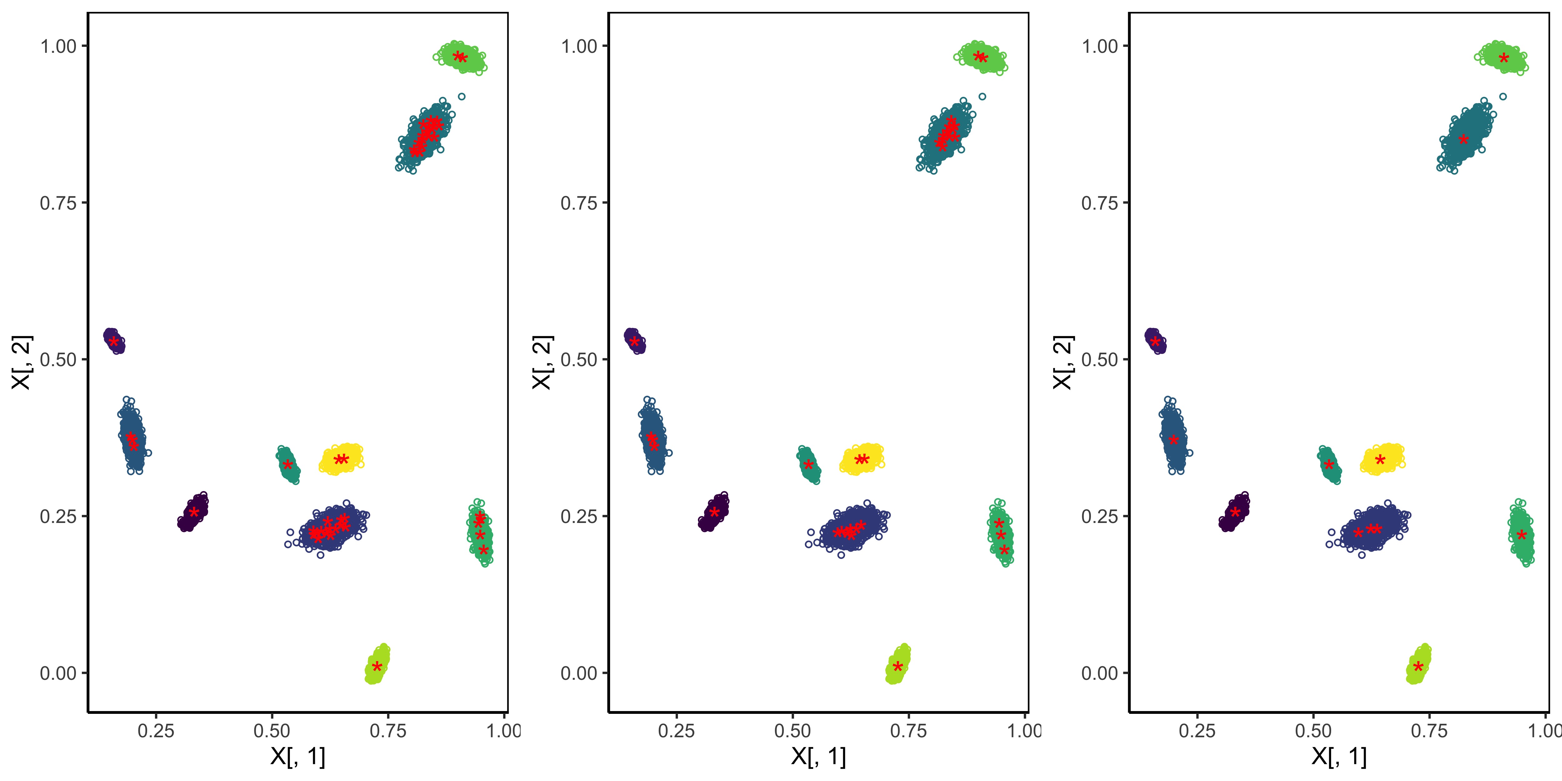
The figure below shows the detected exemplars (red stars) from the density-peak finding method with different settings of the tuning parameters. Well seperated Gaussian components are indicated by different colors. The density-peak finding method detects multiple exemplars for one density peak. An important feature of the REM algorithm is that it produces a decision graph that helps the user select all possible exemplars. We will explore this feature later.
The REM algorithm has two algorithmic blocks: the EM block and the pruning block. Given the updated data pool (the original data without the retained exemplars), the EM block operates as follows.
Input: The retained exemplars $\{\mathbf{e}_1, \ldots, \mathbf{e}_\kappa\}$ and the responsibilities $\{r_{ij}: i=1, \ldots, n, j=1, \ldots, \kappa\}$.
(1) Update the estimates: for $j=1, \ldots, \kappa$, \begin{align*} \pi_j=\frac{\sum_{i=1}^{n}r_{ij}}{n}, ~~~ \mathbf{\Sigma}_j=\frac{\sum_{i=1}^{n}r_{ij}(\mathbf{x}_i-\mathbf{e}_j)(\mathbf{x}_i-\mathbf{e}_j)^T}{\sum_{i=1}^{n}r_{ij}}. \end{align*}
(2) Compute the responsibilities: for $i=1, \ldots, n$ and $j=1, \ldots, \kappa$, \begin{equation*} r_{ij}=\frac{\pi_j\phi(\mathbf{x}_i; \mathbf{e}_j, \mathbf{\Sigma}_j)}{\sum_{v=1}^{\kappa}\pi_v \phi(\mathbf{x}_i; \mathbf{e}_v, \mathbf{\Sigma}_v)}. \end{equation*}
(3) Iterate steps 1 and 2 until convergence.
Output: The mixing proportions $\{\pi_1, \ldots, \pi_\kappa\}$ and the covariance matrices $\{\mathbf{\Sigma}_1, \ldots, \mathbf{\Sigma}_\kappa\}$.
We immediately notice that, in the EM block, the Gaussian means are fixed (at the given exemplars), and we only need to estimate the mixing proportions and covariance matrices. Since the exemplar set is disjoint from the dataset, the mean vectors will always differ from the data points, and therefore the iteration will never converge to a degenerate solution with a zero covariance matrix. The GMM density at convergence is \begin{equation*} f(\mathbf{x})=\sum_{j=1}^{\kappa}\pi_j \phi(\mathbf{x}; \mathbf{e}_j, \mathbf{\Sigma}_j). \end{equation*}
In the pruning block, we remove one exemplar from $\{\mathbf{e}_1, \ldots, \mathbf{e}_\kappa\}$. The idea is to introduce sparsity into the mixing proportion vector $\mathbf{\pi}$ such that, if $\pi_j=0$, then the exemplar $\mathbf{e}_j$ will be removed from the exemplar set (and put back into the data pool).
Input: The covariance matrices $\{\mathbf{\Sigma}_1, \ldots, \mathbf{\Sigma}_\kappa\}$.
(1) Calculate the weight vector $\mathbf{\delta}=(\delta_1, \ldots, \delta_\kappa)^T$: \begin{equation*} \delta_v = \max\left\{\Pr\left(\pi_v\phi(X; \mathbf{e}_v, \mathbf{\Sigma}_v) < \pi_j\phi(X; \mathbf{e}_j, \mathbf{\Sigma}_j) | X \sim N(\mathbf{e}_v, \mathbf{\Sigma}_v )\right): j = 1, \ldots, \kappa, j\neq v\right\},~~~~v=1, \ldots, \kappa. \end{equation*}
(2) Find the $\theta$ value such that the solution to the probem below, i.e., the responsibility matrix $\mathbf{R}=[r_{ij}]_{n\times\kappa}$, has exactly one column of zeros. \begin{align*} \min_{\mathbf{R}} ~~ \left\{\frac{1}{2} \sum_{i=1}^n \sum_{j=1}^{\kappa} r_{ij}(\mathbf{x}_i-\mathbf{e}_j)^T\mathbf{\Sigma}_j^{-1}(\mathbf{x}_i-\mathbf{e}_j) + \frac{1}{2} \sum_{i=1}^n \sum_{j=1}^{\kappa} r_{ij}\log \left(| \mathbf{\Sigma}_j|\right)+\theta\sum_{j=1}^{\kappa} \delta_j(\frac{1}{n}\sum_{i=1}^n r_{ij})\right\}, \\ \mbox{subject to}~~\sum_{j=1}^{\kappa} r_{ij}=1, ~~~i=1, \ldots, n. ~~~~~~~~~~~~~~~~~~~~~~~~~~~~~~~~~~~~~~~~~~~~~~~~~~~~~~~~~~~~~~~~~~~~~~~~~~~~~~~~~~~~~~~~~~ \end{align*}
(3) Remove the exemplar $\mathbf{e}_j$ with $\sum_{i=1}^n r_{ij}=0$ and update $\kappa=\kappa-1$.
Output: The retained exemplars $\{\mathbf{e}_1, \ldots, \mathbf{e}_\kappa\}$ and the responsibilities $\{r_{ij}: i=1, \ldots, n, j=1, \ldots, \kappa\}$.
Both the weight vector $\mathbf{\delta}$ and the penalty function are well-motivatied. The original work Tobin et al. (2023) provides detailed explainations on them. In particular, the conditinal probability $\Pr\left(\pi_v\phi(X; \mathbf{e}_v, \mathbf{\Sigma}_v) < \pi_j\phi(X; \mathbf{e}_j, \mathbf{\Sigma}_j) | X \sim N(\mathbf{e}_v, \mathbf{\Sigma}_v )\right)$ is the likelihood that an instance from the vth mixture component is misclassified into the jth mixture component. Therefore, $\delta_v$ measures the overlapping degree of the vth mixture component w.r.t. the other mixture components. The pruning block is very efficient: (1) the algorithm complexity is linear, and (2) exemplars not representing Gaussian means are always pruned first.
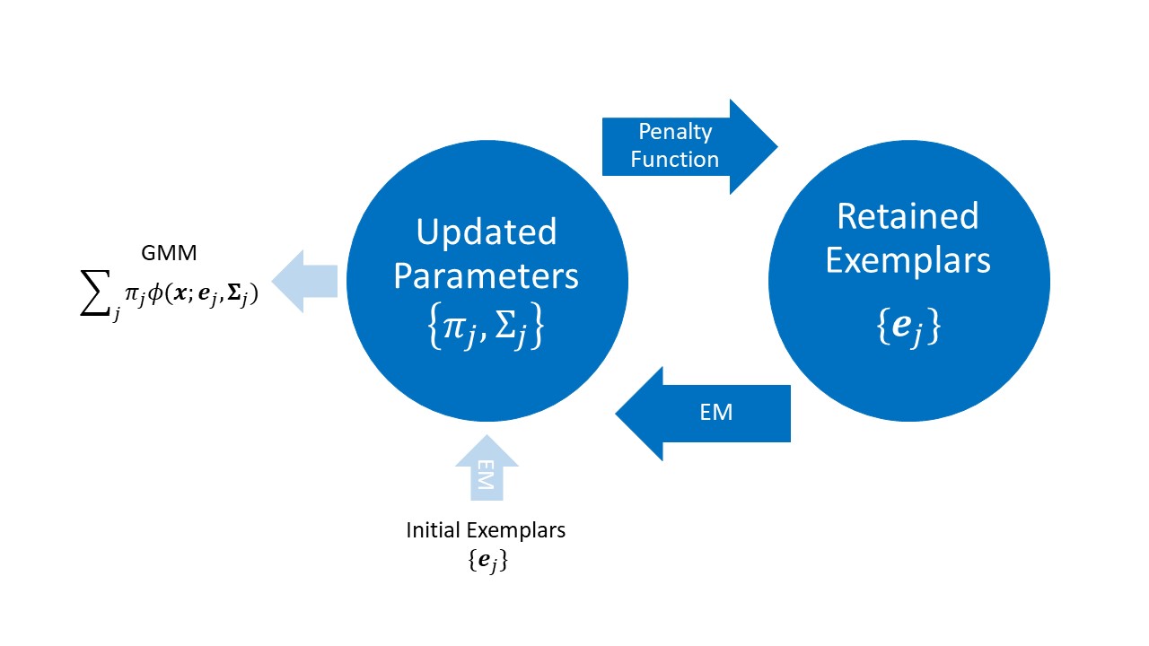
The flowchart below summarizes the REM algorithm. The blue left arrow "EM" means applying the EM block algorithm, and the blue right arrow "Penalty Function" means applying the pruning block algorithm. The loop produces a sequence of nested clusterings, and we pick the optimal clustering via the ICL criterion.
We have implemented our method into the Python package REMclust available at PyPI. The two examples below were contributed by Samuel Singh.
import numpy as np
import matplotlib.pyplot as plt
from sklearn import preprocessing, metrics
from REMclust import REM
import pandas as pd
import seaborn as sns
from sklearn.decomposition import PCA
We apply the REM algorithm to the High Time Resolution Universe Survey (HTRU2) dataset: https://www.kaggle.com/datasets/charitarth/pulsar-dataset-htru2. Pulsars are a rare type of Neutron star that produce radio emission detectable here on Earth. They are of considerable scientific interest as probes of space-time, the interstellar medium, and states of matter. Machine learning tools are now being used to automatically label pulsar candidates to facilitate rapid analysis. In particular, classification systems are widely adopted, which treat the candidate data sets as binary classification problems. Each data point in the HTRU2 dataset is described by 8 variables/features. The target variable is the binary class indicating pulsar candidate.
df = pd.read_csv('Data/HTRU_2.csv')
df.columns = ['µ IRP','σ IRP', 'excess kurtosis IRP', 'skewness IRP',
'µ DM-SNR','σ DM-SNR', 'excess kurtosis DM-SNR', 'skewness DM-SNR',
'class']
X = df[df.columns[:-1]] ## drop the class column
X = np.array(X)
scaler = preprocessing.StandardScaler().fit(X)
X_scaled = scaler.transform(X)
n_samples, n_features = X_scaled.shape
bndwk = int(np.floor(np.min((30, np.sqrt(n_samples)))))
Cluster = REM(data=X_scaled, covariance_type = "full", criteria = "all", bandwidth = bndwk, tol = 1e-3)
Cluster.mode_decision_plot() ## to estimate the density and distance threshold
# Setting the density threshold and distance threshold from the decision plot
Cluster.fit(density_threshold = 1.5, distance_threshold = 3.6)
yp = Cluster.get_labels(mixture_selection='aic') ## predicted labels
2 modes selected.
C:\Users\samue\anaconda3\envs\sisa\lib\site-packages\REMclust\REM.py:432: ComplexWarning: Casting complex values to real discards the imaginary part covariances_jitter[i, :, :] = vec.dot(np.diag(val)).dot(np.linalg.inv(vec))
Match the truth and predicted labels using the Folkes-Mallows index metric and the confusion matrix.
yp = np.where(np.array(yp)==0,1,0) ## corrected yp
# performance metric
fm = metrics.fowlkes_mallows_score(df['class'], yp)
print('Fowlkes-Mallows index (FMI) : %.2f' % (fm))
Fowlkes-Mallows index (FMI) : 0.85
# confusion matrix or classification rate
metrics.ConfusionMatrixDisplay.from_predictions(df['class'], yp, normalize='true')
plt.show()
# pairwise feature plots with predicted cluster labels
df_updated = df[df.columns[:-1]]
df_updated['labels'] = yp
sns.pairplot(df_updated, hue="labels")
plt.show()
pca_X = PCA(n_components=2)
pca_X_scaled = pca_X.fit_transform(X_scaled)
plt.scatter(pca_X_scaled[:, 0], pca_X_scaled[:, 1], s = 5, c = yp, marker = "o", cmap='tab10')
plt.xlabel('Principal Component - 1')
plt.ylabel('Principal Component - 2')
plt.title('PCA')
plt.show()
# NMI & ARI
nmi = metrics.normalized_mutual_info_score(df['class'], yp)
ari = metrics.adjusted_rand_score(df['class'], yp)
print("Adjusted Rand Score: \t", ari)
print("Normalized Mutual Information Score: \t", nmi)
Adjusted Rand Score: 0.3878884708578086 Normalized Mutual Information Score: 0.2743628710506591
# sensitivity w.r.t. density threshold
n = 5
nmi_x = np.zeros((n))
ari_x = np.zeros((n))
dens_thres = [1.3,1.4,1.5,1.6,1.7]
for i in range(n):
Cluster.fit(density_threshold = dens_thres[i],
distance_threshold = 3.6)
yp_x = Cluster.get_labels(mixture_selection='aic')
nmi_x[i] = metrics.normalized_mutual_info_score(df['class'].astype(int), yp_x.astype(int))
ari_x[i] = metrics.adjusted_rand_score(df['class'].astype(int), yp_x.astype(int))
plt.plot(dens_thres, nmi_x, marker = 'o', label='nmi')
plt.plot(dens_thres, ari_x, marker = 'o', label='ari')
plt.xlabel('density threshold')
plt.ylabel('nmi/ari')
plt.legend()
plt.show()
2 modes selected.
C:\Users\samue\anaconda3\envs\sisa\lib\site-packages\REMclust\REM.py:432: ComplexWarning: Casting complex values to real discards the imaginary part covariances_jitter[i, :, :] = vec.dot(np.diag(val)).dot(np.linalg.inv(vec))
2 modes selected.
C:\Users\samue\anaconda3\envs\sisa\lib\site-packages\REMclust\REM.py:432: ComplexWarning: Casting complex values to real discards the imaginary part covariances_jitter[i, :, :] = vec.dot(np.diag(val)).dot(np.linalg.inv(vec))
2 modes selected.
C:\Users\samue\anaconda3\envs\sisa\lib\site-packages\REMclust\REM.py:432: ComplexWarning: Casting complex values to real discards the imaginary part covariances_jitter[i, :, :] = vec.dot(np.diag(val)).dot(np.linalg.inv(vec))
1 modes selected. 1 modes selected.
# sensitivity w.r.t. distance threshold
n = 5
nmi_x = np.zeros((n))
ari_x = np.zeros((n))
dist_thres = [3.4,3.5,3.6,3.7,3.8]
for i in range(n):
Cluster.fit(density_threshold = 1.5,
distance_threshold = dist_thres[i])
yp_x = Cluster.get_labels(mixture_selection='aic')
nmi_x[i] = metrics.normalized_mutual_info_score(df['class'].astype(int), yp_x.astype(int))
ari_x[i] = metrics.adjusted_rand_score(df['class'].astype(int), yp_x.astype(int))
plt.plot(dist_thres, nmi_x, marker = 'o', label='nmi')
plt.plot(dist_thres, ari_x, marker = 'o', label='ari')
plt.xlabel('density threshold')
plt.ylabel('nmi/ari')
plt.legend()
plt.show()
2 modes selected.
C:\Users\samue\anaconda3\envs\sisa\lib\site-packages\REMclust\REM.py:432: ComplexWarning: Casting complex values to real discards the imaginary part covariances_jitter[i, :, :] = vec.dot(np.diag(val)).dot(np.linalg.inv(vec))
2 modes selected.
C:\Users\samue\anaconda3\envs\sisa\lib\site-packages\REMclust\REM.py:432: ComplexWarning: Casting complex values to real discards the imaginary part covariances_jitter[i, :, :] = vec.dot(np.diag(val)).dot(np.linalg.inv(vec))
2 modes selected.
C:\Users\samue\anaconda3\envs\sisa\lib\site-packages\REMclust\REM.py:432: ComplexWarning: Casting complex values to real discards the imaginary part covariances_jitter[i, :, :] = vec.dot(np.diag(val)).dot(np.linalg.inv(vec))
1 modes selected. 1 modes selected.
Our next dataset is the Palmer Archipelago (Antarctica) Penguin Dataset: https://www.kaggle.com/datasets/parulpandey/palmer-archipelago-antarctica-penguin-data for studying three species of penguins: Adelie Penguins (Pygoscelis adeliae), Gentoo Penguins (Pygoscelis papua), and Chinstrap Penguins (Pygoscelis antarctica). Each data point in the Penguin dataset is described by 4 variables/features. The target variable is the species class, which includes the three aforementioned species of penguins.
df = pd.read_csv('Data/penguins_size.csv')
df['species'] = df['species'].map({'Adelie':0, 'Gentoo':1, 'Chinstrap':2}) ## for one hot encoding
df['island'] = df['island'].map({'Torgersen':0, 'Biscoe':1, 'Dream':2})
df['sex'] = df['sex'].map({'MALE':0, 'FEMALE':1})
df = df.dropna() ## to discard nan value datapoints
X = df[df.columns[2:-1]] ## considering the length and depth of beak, flipper length and body mass
X = np.array(X)
scaler = preprocessing.StandardScaler().fit(X)
X_scaled = scaler.transform(X)
n_samples, n_features = X_scaled.shape
bndwk = int(np.floor(np.min((30, np.square(n_samples)))))
Cluster = REM(data=X_scaled, covariance_type = "full", criteria = "all", bandwidth = bndwk, tol = 1e-3)
Cluster.mode_decision_plot()
# Setting the density threshold and distance threshold from the decision plot
Cluster.fit(density_threshold = 1.15, distance_threshold = 1.00)
yp = Cluster.get_labels(mixture_selection='aic')
3 modes selected.
The predicted clusters are labeled with '0', '1', and '2'. Based on the confusion matrix, it can be deduced that the predicted label '1' corresponds to the ground truth '2', and vice versa. Accordingly, appropriate corrections are made.
yp[yp == 2] = 3; yp[yp == 1] = 2; yp[yp == 3] = 1; ## corrected yp
# performance metric
fm = metrics.fowlkes_mallows_score(df['species'], yp)
print('Fowlkes-Mallows index (FMI) : %.2f' % (fm))
Fowlkes-Mallows index (FMI) : 0.85
# confusion matrix or classification rate
metrics.ConfusionMatrixDisplay.from_predictions(df['species'], yp, normalize='true')
plt.show()
# pairwise feature plots
df_updated = df[df.columns[2:-1]]
df_updated = df_updated.assign(labels=yp)
sns.pairplot(df_updated, hue="labels", palette='tab10')
plt.show()
pca_X = PCA(n_components=2)
pca_X_scaled = pca_X.fit_transform(X_scaled)
plt.scatter(pca_X_scaled[:, 0], pca_X_scaled[:, 1], s = 5, c = yp, marker = "o", cmap='tab10')
plt.xlabel('Principal Component - 1')
plt.ylabel('Principal Component - 2')
plt.title('PCA')
plt.show()
# NMI & ARI
nmi = metrics.normalized_mutual_info_score(df['species'].astype(int), yp.astype(int))
ari = metrics.adjusted_rand_score(df['species'].astype(int), yp.astype(int))
print("Adjusted Rand Score: \t", ari)
print("Normalized Mutual Information Score: \t", nmi)
Adjusted Rand Score: 0.7740574481288712 Normalized Mutual Information Score: 0.7785511759363766
# sensitivity w.r.t. density threshold
n = 5
nmi_x = np.zeros((n))
ari_x = np.zeros((n))
dens_thres = [1.05,1.10,1.15,1.20,1.25]
for i in range(n):
Cluster.fit(density_threshold = dens_thres[i],
distance_threshold = 1.0)
yp_x = Cluster.get_labels(mixture_selection='aic')
nmi_x[i] = metrics.normalized_mutual_info_score(df['species'].astype(int), yp_x.astype(int))
ari_x[i] = metrics.adjusted_rand_score(df['species'].astype(int), yp_x.astype(int))
plt.plot(dens_thres, nmi_x, marker = 'o', label='nmi')
plt.plot(dens_thres, ari_x, marker = 'o', label='ari')
plt.xlabel('density threshold')
plt.ylabel('nmi/ari')
plt.legend()
plt.show()
3 modes selected. 3 modes selected. 3 modes selected. 2 modes selected. 2 modes selected.
# sensitivity w.r.t. distance threshold
n = 5
nmi_x = np.zeros((n))
ari_x = np.zeros((n))
dist_thres = [0.90,0.95,1.00,1.05,1.10]
for i in range(n):
Cluster.fit(density_threshold = 1.0,
distance_threshold = dist_thres[i])
yp_x = Cluster.get_labels(mixture_selection='aic')
nmi_x[i] = metrics.normalized_mutual_info_score(df['species'].astype(int), yp_x.astype(int))
ari_x[i] = metrics.adjusted_rand_score(df['species'].astype(int), yp_x.astype(int))
plt.plot(dist_thres, nmi_x, marker = 'o', label='nmi')
plt.plot(dist_thres, ari_x, marker = 'o', label='ari')
plt.xlabel('distance threshold')
plt.ylabel('nmi/ari')
plt.legend()
plt.show()
3 modes selected. 3 modes selected. 3 modes selected. 2 modes selected. 2 modes selected.
The math behind the REM algorithm may not be straightforward for engineers. But the algorithm and the Python library do not need much manual input. On the contrary, it has the additional feature (the desion graph) to help select all possible exemplars.
(1) Tobin, J., Ho, C.P., and Zhang, M. (2023). Reinforced EM Algorithm for Clustering with Gaussian Mixture Models, In Proceedings of the 2023 SIAM International Conference on Data Mining (SDM 2023).
(2) Bishop, C. (2006). Pattern Recognition and Machine Learning. Information Science and Statistics. Springer-Verlag New York, 1st edition.
(3) Jin, C., Zhang, Y., Balakrishnan, S., Wainwright, M. J., and Jordan, M. I. (2016). Local Maxima in the Likelihood of Gaussian Mixture Models: Structural Results and Algorithmic Consequences. In Proceedings of the 30th International Conference on Neural Information Processing Systems (NIPS 2016).